
In today’s era of machine learning and advanced algorithms, interpreting model results plays a crucial role. Traditional algorithms like linear regression and logistic regression are not only good for making predictions but also make it easy to understand how each feature affects the outcome.
However, modern machine learning models—especially tree-based ensemble methods—often behave like “black boxes.” They deliver strong predictive performance, but it becomes difficult to understand what is happening inside the model.
In recent years, several techniques have been developed to help interpret the results of these complex models. SHAP (SHapley Additive exPlanations) is one of the most powerful and widely adopted methods. Although SHAP is extremely useful, many people in the industry are still not fully aware of how it works or how to use it effectively.
In this article, we will explore the basic idea of SHAP and understand how it helps in interpreting machine learning models.
What are SHAP values?
SHAP is a methodology used for the interpretation of machine learning models. SHAP helps us identify features that contribute positively, negatively, or neutrally to a model’s prediction. It uses a game theory–based approach to determine the contribution of each feature to the final model output.
SHAP helps us understand a model’s prediction by showing:
Which features influenced the prediction
How much each feature contributed to the final outcome
Whether the contribution was positive, negative or neutral
Characteristic of SHAP values
Model-Agnostic
SHAP values work with any machine learning algorithm like Linear regression, decision trees, random forest etc
Additive Explanation
Final model prediction is actually the sum of all SHAP values along with models base line prediction
Local Interpretability
SHAP is capable of providing explanation for even a single data point
Fair Feature Attribution
SHAP splits the credit fairly among all features based on how important each one actually was
Implementation of SHAP values in Python
By the end of this walkthrough, you will be able to:
Understand the essential Python libraries used to build a machine learning model and interpret its predictions
Import a dataset and train a predictive model
Identify the top contributing features influencing the model’s output
Determine which features contribute positively and which contribute negatively to the prediction
Interpret individual data points to understand how the model arrived at a specific outcome
Dataset Description
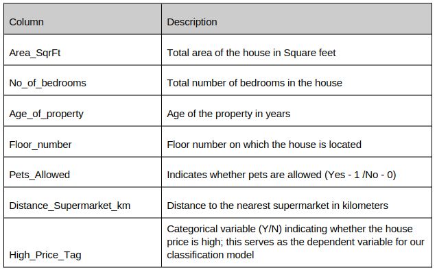
In this walkthrough, we use a simulated dataset containing information on approximately 10,000 houses. The target variable, High_Price_Tag (Yes/No), indicates whether a house is considered high-priced. This variable serves as the dependent variable and is predicted using a set of independent features related to house characteristics.
The dataset contains the following fields:
Let’s start by building a model in Python.
Step 1 : Import essential libraries and the dataset
Begin by importing the necessary libraries such as pandas, matplotlib, shap and relevant modules from scikit-learn (sklearn).
#------------------------------------------
#Set datapath and import required libraries
#------------------------------------------

import pathlib
from pathlib import Path
base_path = Path.cwd()/"Data"

import shap
import pandas as pd
import numpy as np
import matplotlib.pyplot as plt
from sklearn.model_selection import train_test_split
from sklearn.ensemble import RandomForestClassifier
from sklearn.metrics import confusion_matrix, accuracy_score, classification_report

#------------------------------------------
#import data
#------------------------------------------
file = base_path / "Housing_Price_Data.csv"
df_housing_base = pd.read_csv(file)
Step 2: Build the random forest model
In this step, we define the dependent variable and the independent variables. Using these variables, we then train a basic Random Forest classification model to predict whether a house falls into the high-price category.
# Define dependent and independent variables
y = df_housing_base["High_Price_Tag"]
X = df_housing_base.drop(['High_Price_Tag'], axis = 1)
# Train and Test Split
X_train, X_test, y_train, y_test = train_test_split(X, y, test_size=0.2, random_state=25)

#Build model

clf = RandomForestClassifier()
clf.fit(X_train, y_train)

# Classification Report
print(classification_report(y_pred, y_test))
Output :
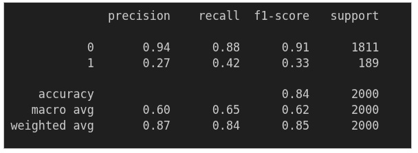
The classification report indicates that the model has performed reasonably well.
Now, let’s move on to interpreting the model’s predictions.
Step 3: Identify the top contributing features
In this step, we initialize SHAP to interpret the trained model and identify the most influential features. Using a SHAP summary plot, we can visualize the top contributing features and understand their overall impact on the model’s predictions.
shap.initjs()

# Calculate SHAP values
explainer = shap.TreeExplainer(clf)
shap_values = explainer.shap_values(X_test)

shap.summary_plot(shap_values[:,:,1], X_test, plot_type="bar")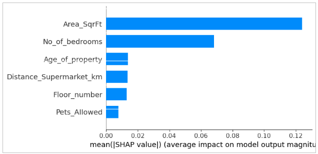
‘Area_SqrFt’ is the most influential feature, followed by ‘No_of_bedrooms’ .
Step 4 : Understand how feature values contribute to the model
Next, we examine how individual feature values contribute to the model’s predictions. This step helps us understand whether specific feature values have a positive or negative impact on the model’s outcome and the direction in which they influence the prediction.
shap.summary_plot(shap_values[:, :, 1], X_test)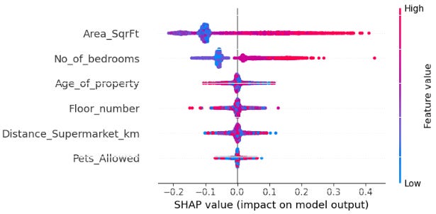
In the SHAP summary plot, red indicates higher feature values, while blue represents lower feature values.
For example, in the case of Area_SqrFt, higher area values are shown in red and lower values in blue. From the plot, we observe that the SHAP value increases as the area of the property increases. This indicates that larger properties are more likely to be classified as high-value by the model.
Examining the Floor_number feature, we observe an opposite trend. Higher floor numbers tend to have negative SHAP values, suggesting that properties located on higher floors are more likely to be classified as low-value by the model.
Step 5 : Interpret an individual data point
In this step, we interpret how the model arrived at a specific prediction for an individual observation. Specifically, we analyze row number 1999 using a SHAP force plot to understand how each feature contributed to the final model output.
shap.plots.force(explainer.expected_value[1], shap_values[:, :, 1][1998,:], X_test.iloc[1998, :], matplotlib = True)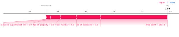
For row number 1,999, we observe that a larger area (square footage) and a higher number of bedrooms push the model’s prediction toward a higher property price.
Conclusion
Interpreting model results is just as important as building a high-performing model. SHAP values provide a powerful and intuitive way to understand model predictions. They not only highlight the most influential features but also reveal how individual feature values contribute positively or negatively to the model’s outcomes. By leveraging SHAP, we can gain transparency, build trust in the model, and make more informed decisions based on its predictions.